Sigma-Epsilon Diagram

Contents
A Sigma-Epsilon diagram, also known as a stress-strain diagram, graphically represents the relationship between stress (σ) and strain (ε) for a material under load. This diagram helps to understand how a material behaves under different levels of stress and strain.

This diagram typically includes the following regions:
•Elastic Region (O-A): The initial linear portion where the material deforms elastically. Stress and strain are proportional, and the material returns to its original shape when the load is removed.
•Yield Point: The point where the material begins to deform plastically. Beyond this point, the material will not return to its original shape. There are 2 yield points: upper yield point (B) and lower yield point (C).
•Plastic Region (B-E): The non-linear portion where permanent deformation occurs.
•Ultimate Strength (D): The maximum stress the material can withstand.
•Fracture Point (E): The point where the material ultimately breaks.
Once the Material Non-Linear Model option is selected, the actual stress-strain relationship, defined using the input tables ISTROP and SIGEPS in Design Function 3.1, can be displayed in a Sigma-Epsilon diagram.

An example of a Sigma-Epsilon diagram in PLE
The output tables PIPEMAT and PIPEPLS in Design Function 3.1 will have an extra button in the table toolbar.
Standard toolbar: |
|
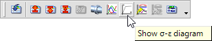
Sigma-Epsilon toolbar: |
|
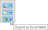
Having the graph on screen there is an extra button to export the underlying data to Excel:
Standard toolbar: |
|
Sigma-Epsilon toolbar: |
|

![]() Calculating material-linear, the diagram will show a straight line.
Calculating material-linear, the diagram will show a straight line.
This also counts for anisotropic materials, because they are always calculated material-linear.
H3105 (last modified: Sep 22, 2025)
See also: